Neural Stochastic Optimal Control

Problem statement

Numerical optimal control solvers efficiently compute locally optimal trajectories given smooth and differentiable objective functions. Conversely, RL approximates general policies while using sampling to relax differentiability requirements on the objective.

Aim. Formulate a global method that uses sampling to handle discontinuities inspired by RL while preserving efficiency and generalisation.

Continuous stochastic Bellman equation

In this case, we use the stochastic HJB equation.

\[ -\frac{\partial v\left(\vec x_t,t\right)}{\partial t}=\min_{\vec u_t}\left[\ell\left(\vec x_t,\vec u_t\right)+\nabla_{\vec x_t}v\left(\vec x_t,t\right)\vec f\left(\vec x_t,\vec u_t\right)+\frac{1}{2}\operatorname{trace}\left(\nabla^2_{\vec x_t\vec x_t}v\left(\vec x_t,t\right)\vec\Sigma\left(\vec x_t\right)\right)\right] \]

Optimal controls. Assuming affine control \(d\vec x_t=\left(\vec h\left(\vec x_t\right)+\vec g\left(\vec x_t\right)\vec u_t\right)\,dt+\vec B\left(\vec x_t\right)\,d\vec w_t\) and quadratic control cost, we can analytically solve for \(\vec u_t\):

\[ \vec u^*\left(\vec x_t\right)=-\left(\nabla^2_{\vec u_t}\ell_{\text{ctrl}}\left(\vec u_t\right)\right)^{-1}\left(\nabla_{\vec x_t}v\left(\vec x_t,t\right)\nabla_{\vec u_t}\vec f\left(\vec x_t,\vec u_t\right)\right) \]

Our optimal control remains the same, and so does our choice of parameterisation: the value function.

Learning the value function

As in the deterministic case, we define a constraint on the expected rate of change of value function.

\[ \begin{aligned} \mathbb E_{\mathcal Q}\left[\frac{dv\left(\vec x_t,t\right)}{dt}\right]&=-\ell\left(\vec x_t,\vec u_t^*\right)\\ \mathbb E_{\mathcal Q}\left[v\left(\vec x_t,t\right)-v\left(\vec x_{t+\Delta t},t+\Delta t\right)\right]&=\ell\left(\vec x_t,\vec u_t^*\right)\Delta t\\ v\left(\vec x_t,t\right)-\mathbb E_{\mathcal Q}\left[v\left(\vec x_{t+\Delta t},t+\Delta t\right)\right]&=\ell\left(\vec x_t,\vec u_t^*\right)\Delta t \end{aligned} \]

Intuition. Under policy \(\vec u_t^*\), the expected change in value equals the negative cost rate in expectation.

TD(ish) view

Satisfying this constraint over horizon \(N\) can be viewed through an update analogous to TD.

\[ \begin{aligned} \mathbb E_{\mathcal Q}\left[v\left(\vec x_N,N\right)\right]-\mathbb E_{\mathcal Q}\left[\psi\left(\vec x_N\right)\right]&=0\\ v\left(\vec x_{N-1},N-1\right)-\mathbb E_{\mathcal Q}\left[v\left(\vec x_N,N\right)\right]-\ell\left(\vec x_{N-1},\vec u^*_{N-1}\right)\Delta t&=0\\ v\left(\vec x_{N-2},N-2\right)-\mathbb E_{\mathcal Q}\left[v\left(\vec x_{N-1},N-1\right)\right]-\ell\left(\vec x_{N-2},\vec u^*_{N-2}\right)\Delta t&=0\\ &\vdots\\ v\left(\vec x_0,0\right)-\mathbb E_{\mathcal Q}\left[v\left(\vec x_1,1\right)\right]-\ell\left(\vec x_0,\vec u^*_0\right)\Delta t&=0 \end{aligned} \]

Note. We cannot simply sum costs backwards because of the expectation under \(\mathcal Q\).

Gradient computation

Stochastic adjoints are costly here, so we reparameterise the Euler-Maruyama step with Gaussian noise, approximate the expectation by Monte Carlo, and backpropagate through the sampled rollout.

\[ \begin{aligned} \vec x_{i+1}\left(\theta,\vec \epsilon_i\right)&=\vec x_i+\left(\vec h\left(\vec x_i\right)+\vec g\left(\vec x_i\right)\vec u_i^*\right)\Delta t+\vec B\left(\vec x_i\right)\vec \epsilon_i\sqrt{\Delta t},\qquad \vec \epsilon_i\sim\mathcal N\left(0,\vec I\right)\\ \nabla_\theta \mathbb E_{\mathcal Q}\left[v\left(\vec x_{i+1},i+1;\theta\right)\right]&\approx\mathbb E_{\vec \epsilon}\left[\nabla_\theta v\left(\vec x_{i+1}\left(\theta,\vec \epsilon_i\right),i+1;\theta\right)\right] \end{aligned} \]

Intuition. Noise is sampled, not differentiated; gradients flow through the sampled next state and the Bellman residual.

Discrete algorithm

Initialize: x(0)=x₀, Δt, N=T/Δt, E_Q[v(x_N,N)] = E_Q[ψ(x_N)]
For i = 0 ... N−1:
  u_i = −(∇²_{u_i} l_ctrl(u_i))⁻¹ g(x_i)^T ∇_x ṽ(x_i, i; θ)^T
  x_i+1 = x_i + ( h(x_i) + g(x_i)u_i ) Δt + B(x_i) ε_i √Δt
Optimize: min_θ Σ_i=0..N ( ṽ(x_i, i, θ) − E_Q[ṽ(x_i+1, i+1, θ)] − l(x_i, u_i^*) Δt )²

Intuition. Roll out trajectories under the current optimal policy, then fit the stochastic Bellman residual.

Results

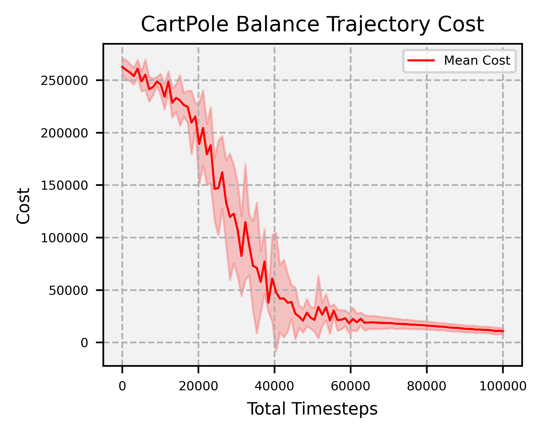
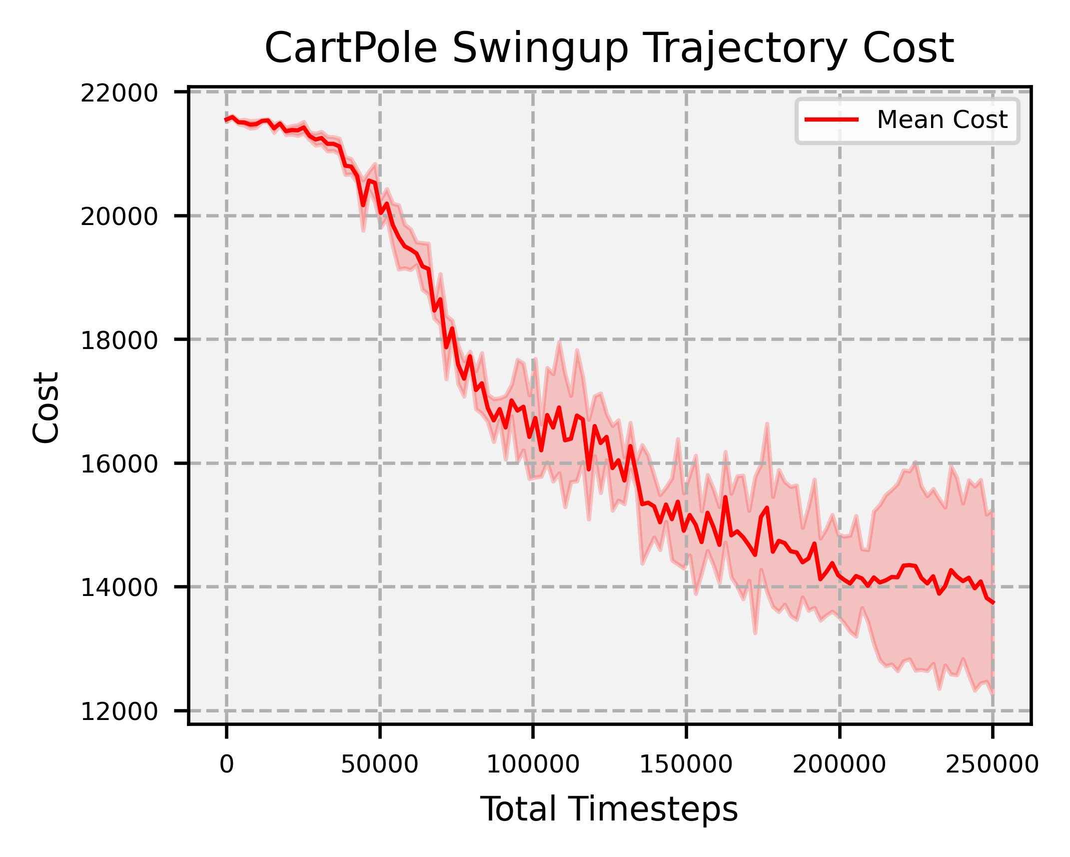
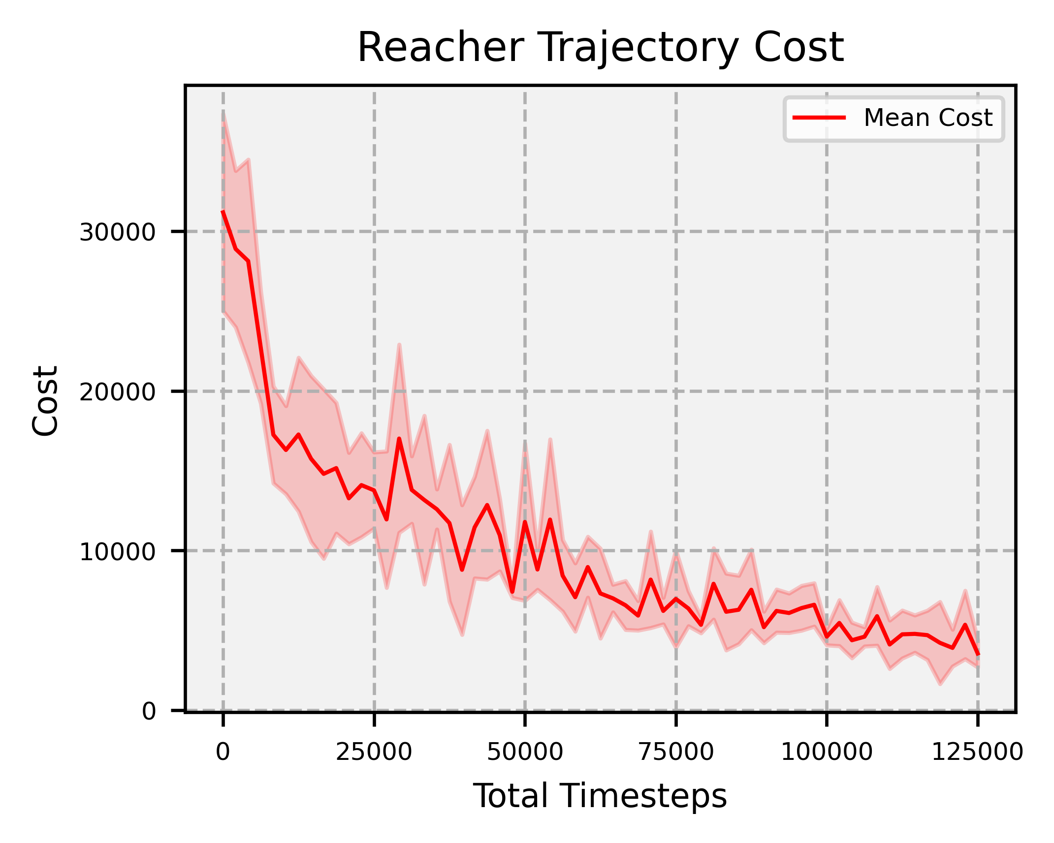
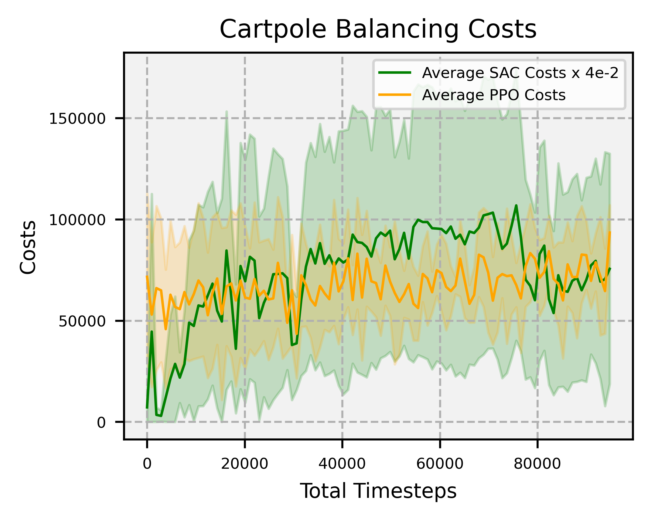
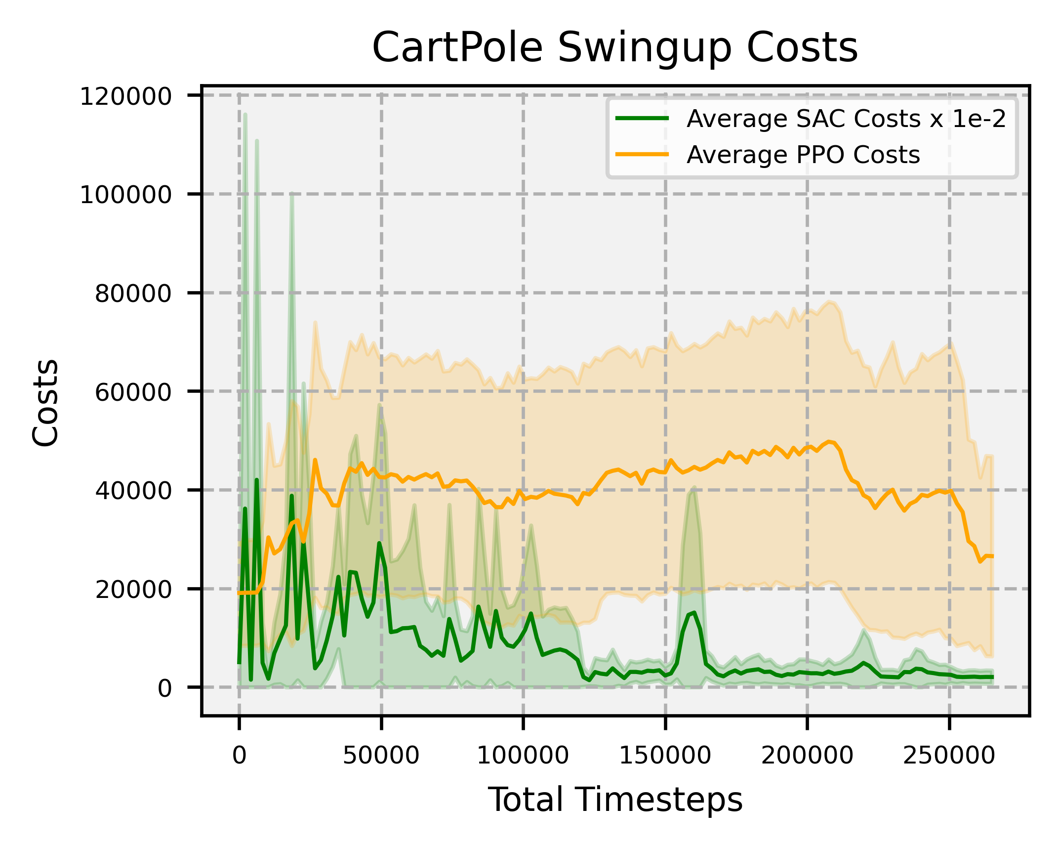
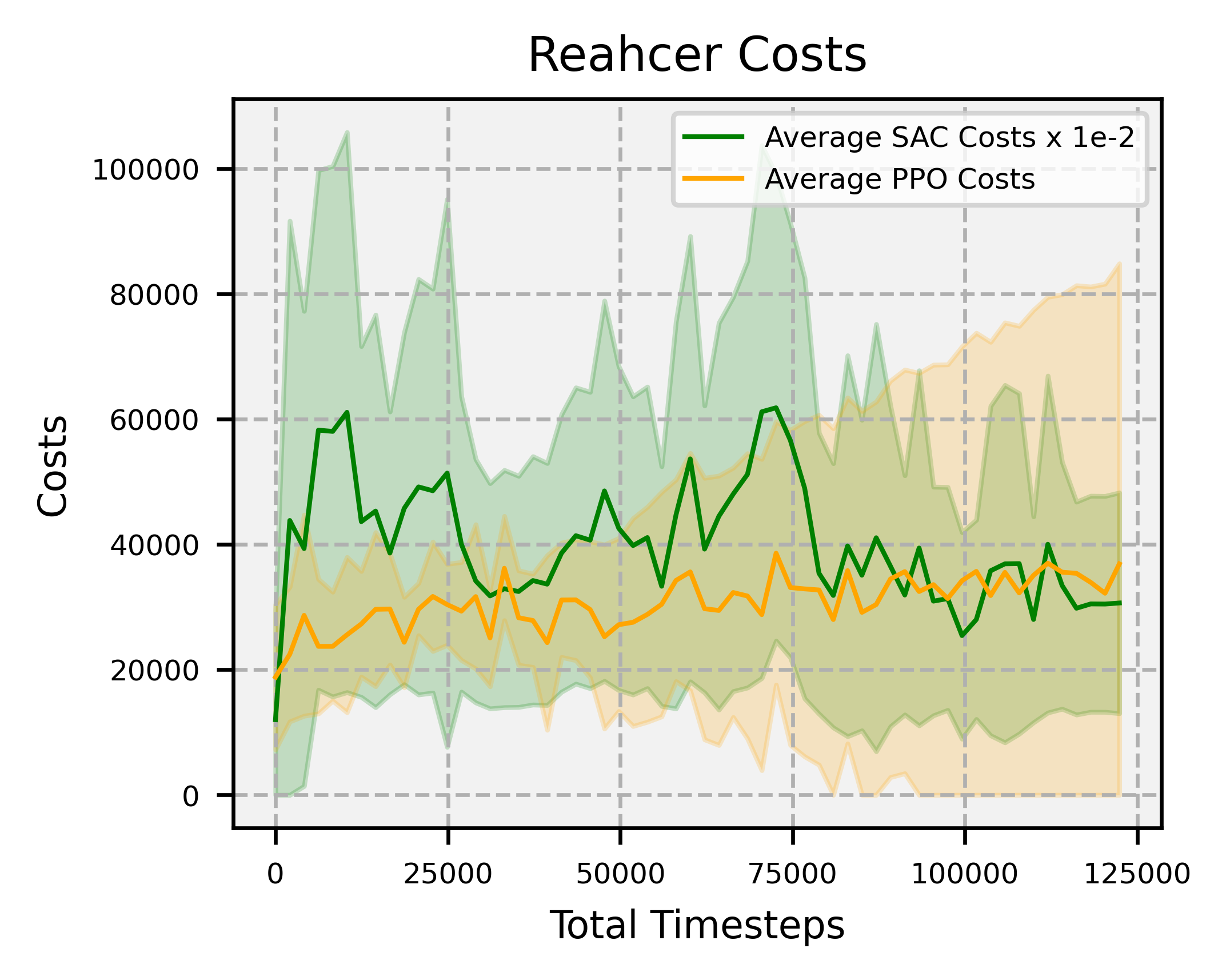
Stochastic cartpole balance trajectory cost

Stochastic cartpole swingup trajectory cost

Overview: significantly faster convergence and lower variance across random seeds, outperforming SAC and PPO by at least factors of 18 and 2, respectively.

Noise-driven smoothing (Obstacle avoidance with discontinuous objective)

Value learning under stochastic dynamics and discontinuous objectives.

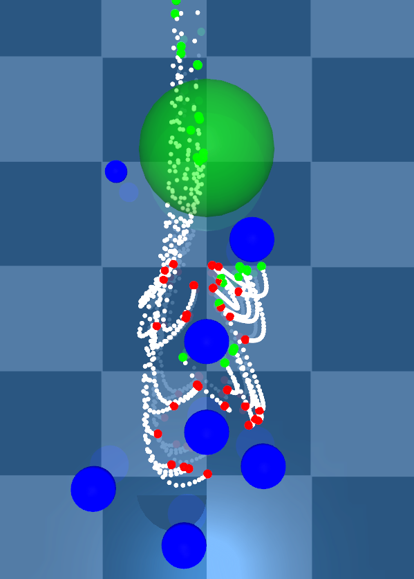
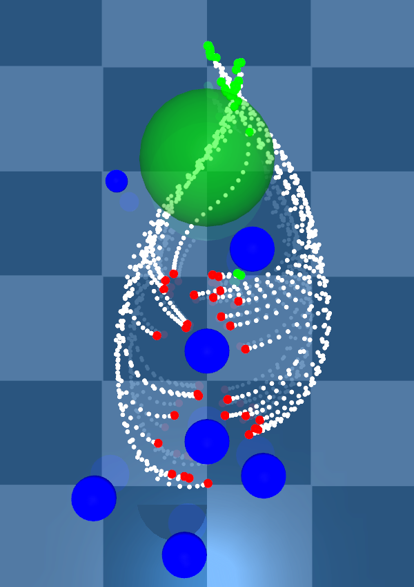
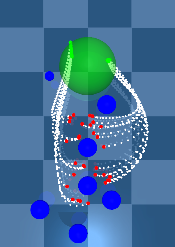
Higher noise regularises the value function through the curvature term \(\operatorname{trace}\left(\nabla^2_{\vec x_t\vec x_t}v\left(\vec x_t,t\right)\vec\Sigma\left(\vec x_t\right)\right)\).

As we increase the control noise samples move trajectories farther from obstacles. This is evidence that noise regularises value function curvature, improving robustness.