Neural Lyapunov and Optimal Control

Problem statement

Numerical optimal control solvers parameterise trajectories to provide locally optimal solutions given smooth and differentiable objective functions. Conversely, RL parameterises function space to synthesise approximate global policies.

Aim. Combine the generalisation capabilities of RL with the efficiency of OC theoretic solutions by leveraging differentiation for efficiency and function-space parameterisation for generalisation.

Optimisation in RL

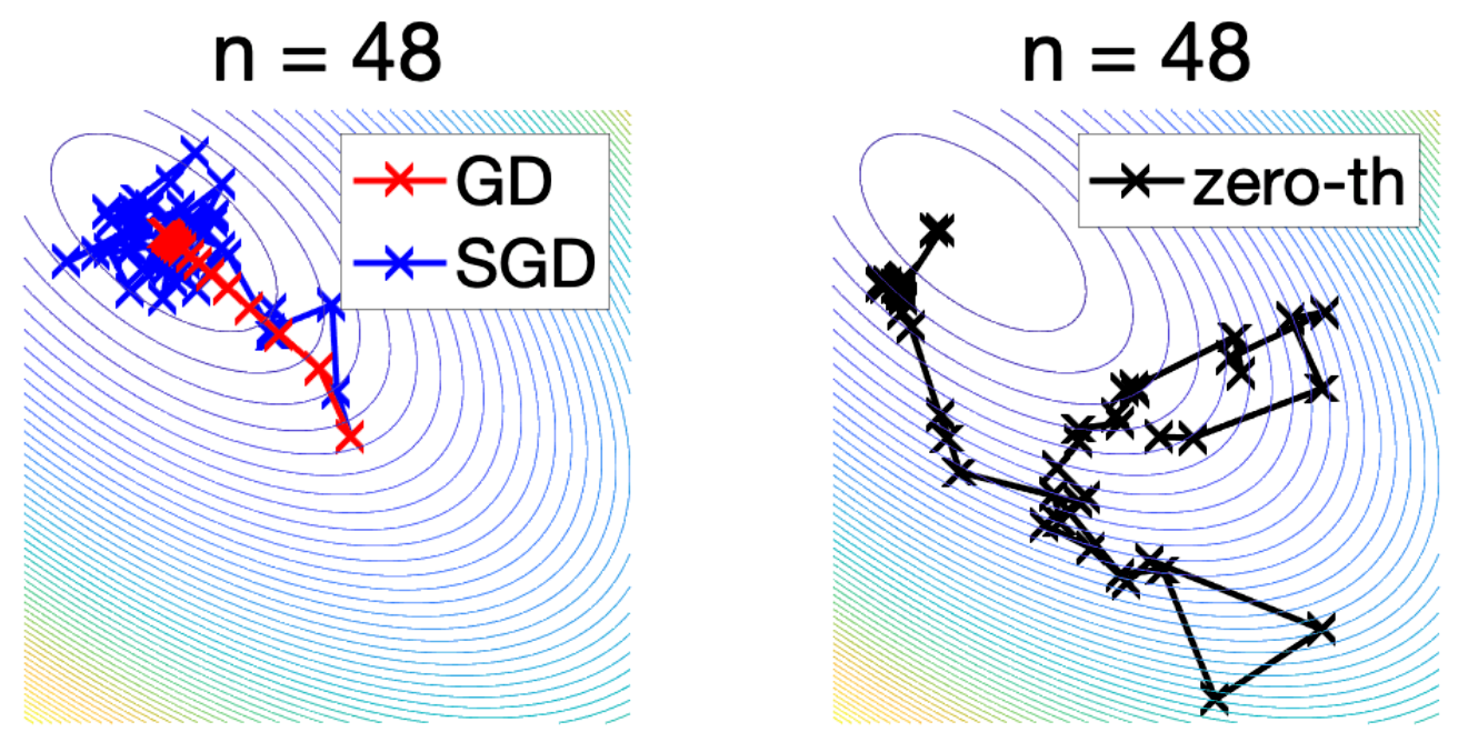
Famous RL environments

RL environments tinker with dynamics tuning under the hood.

Continuous Bellman equation

Our approach relies on the Hamilton-Jacobi-Bellman equation.

\[ -\frac{\partial v}{\partial t}\left(\vec{x}_t,t\right)=\operatorname*{min}_{\vec u\in\vec U}\left[\ell\left(\vec{x}_t,\vec{u}_t\right)+\vec f\left(\vec{x}_t,\vec{u}_t\right)^\top\nabla_{\vec x_t}v\left(\vec{x}_t,t\right)^\top\right] \]

Optimal controls. Assuming affine control \(\dot{\vec x}_t=\vec h\left(\vec x_t\right)+\vec g\left(\vec x_t\right)\vec u_t\) and quadratic control cost, we can solve analytically:

\[ \vec u^*\left(\vec x_t\right)=-\left(\nabla^2_{\vec u_t}\ell_{\text{ctrl}}\left(\vec u_t\right)\right)^{-1}\left(\nabla_{\vec x_t}v\left(\vec x_t,t\right)\nabla_{\vec u_t}\vec f\left(\vec x_t,\vec u_t\right)\right) \]

This computes the optimal greedy control given the optimal value function, motivating value-function parameterisation.

Local solutions

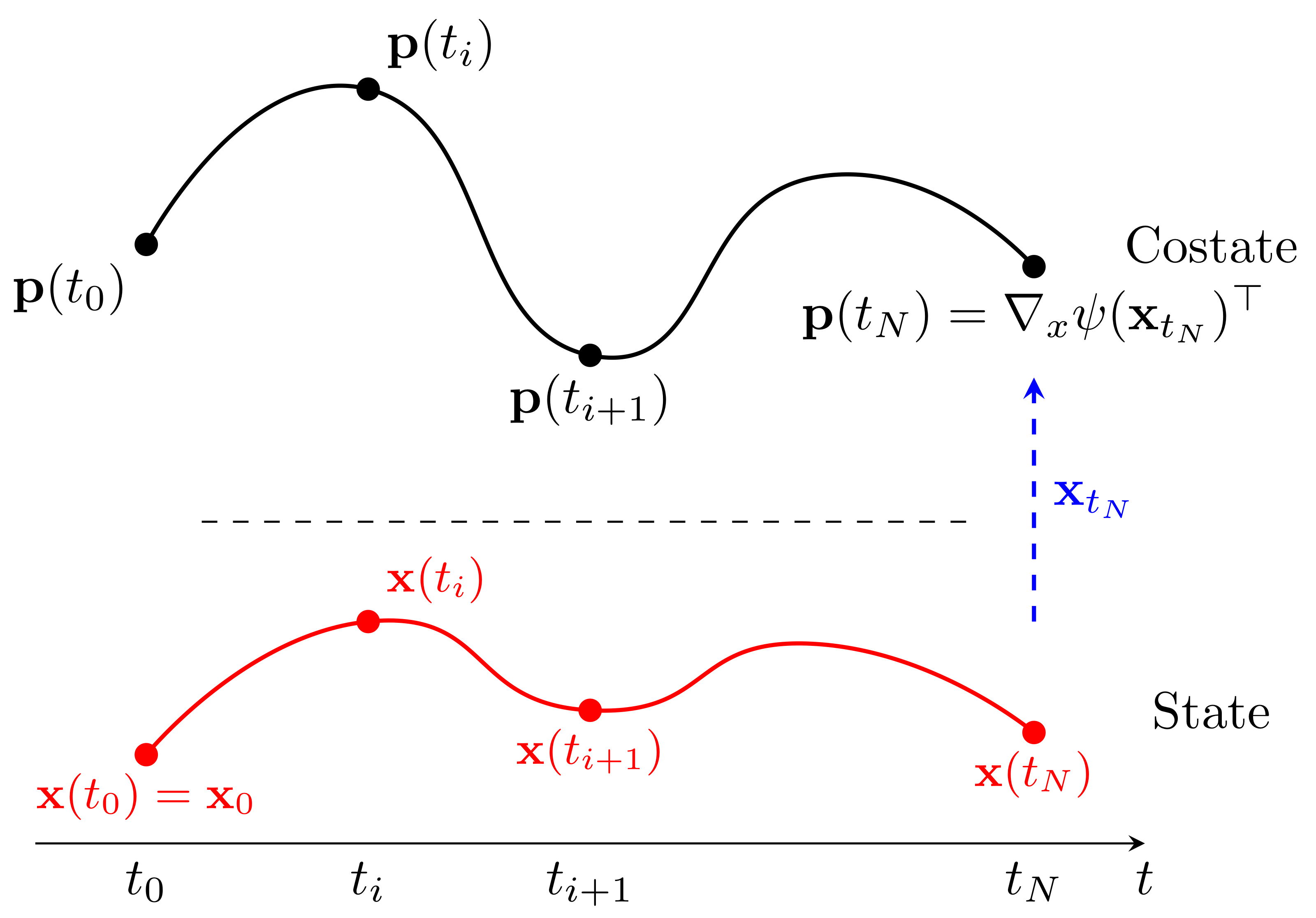
Pontryagin's minimum principle is the classical local trajectory-space solution and the basis for methods such as DDP and iLQR.

\[ \begin{aligned} \dot{\vec x} &= \vec f\left(\vec x_t,\vec u_t\right)\\ \dot{\vec p} &= -\nabla_{\vec x_t}\ell\left(\vec x_t,\vec u_t\right)-\nabla_{\vec x_t}\vec f^\top\left(\vec x_t,\vec u_t\right)\vec p\left(t\right)\\ \vec u^* &= -\left(\nabla^2_{\vec u_t}\ell_{\text{ctrl}}\left(\vec u_t\right)\right)^{-1}\left(\vec g\left(\vec x_t\right)^\top\vec p\left(t\right)\right) \end{aligned} \]

Initial condition: \(\vec x=\vec x_0\in\mathbb{R}^m\). Terminal condition: \(\vec p\left(T\right)=\nabla_{\vec x_T}\psi\left(\vec x_T\right)^\top\).

PMP

Solve one ODE forward for \(\vec x(t)\) and one backward for \(\vec p(t)\).

Making PMP global

Rearranging HJB gives a concise constraint on the rate of change of the value function:

\[ \begin{aligned} \frac{\partial v}{\partial t}\left(\vec x_t,t\right)+\nabla_{\vec x_t}v\left(\vec x_t,t\right)\frac{d\vec x_t}{dt}&=-\ell\left(\vec x_t,\vec u_t^*\right)\\ \frac{dv\left(\vec x_t,t\right)}{dt}&=-\ell\left(\vec x_t,\vec u_t^*\right) \end{aligned} \]

Intuition. Under policy \(\vec u_t^*\), value decreases at a rate negative to cost.

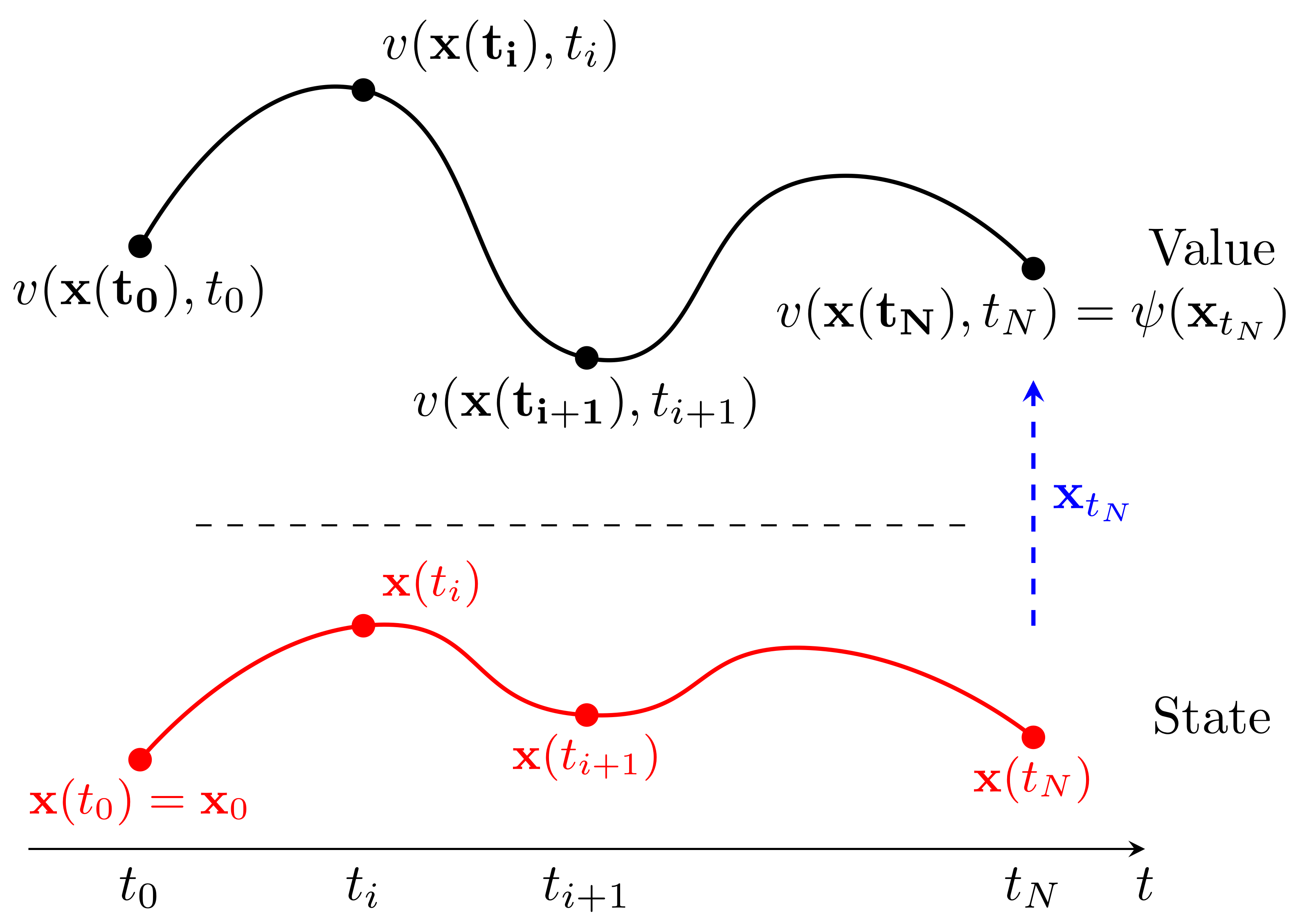
Making PMP global (parameterised value function)

Parameterise \(v\left(\vec x_t,t;\theta\right)\) directly to learn an approximate global value function and therefore policy.

\[ \begin{aligned} \dot{\vec x} &= \vec f\left(\vec x_t,\vec u_t\right)\\ \dot v &= -\ell\left(\vec x_t,\vec u_t\right)\\ \vec u^* &= -\left(\nabla^2_{\vec u_t}\ell_{\text{ctrl}}\left(\vec u_t\right)\right)^{-1}\left(\vec g\left(\vec x_t\right)^\top\nabla_{\vec x_t}v\left(\vec x_t,t;\theta\right)\right) \end{aligned} \]

Initial: \(\vec x=\vec x_0\in\mathbb{R}^{B\times m}\). Terminal: \(v\left(\vec x_T,T;\theta\right)=\psi\left(\vec x_T\right)\).

Dynamic programming view

The discrete solution resembles a dynamic programming update:

\[ \begin{aligned} v\left(\vec x_N,N\right)&=\psi\left(\vec x_N\right)\\ v\left(\vec x_{N-1},N-1\right)&=v\left(\vec x_N,N\right)+\ell\left(\vec x_{N-1},\vec u^*_{N-1}\right)\Delta t\\ v\left(\vec x_{N-2},N-2\right)&=v\left(\vec x_{N-1},N-1\right)+\ell\left(\vec x_{N-2},\vec u^*_{N-2}\right)\Delta t\\ &\vdots\\ v\left(\vec x_0,0\right)&=v\left(\vec x_1,1\right)+\ell\left(\vec x_0,\vec u^*_0\right)\Delta t \end{aligned} \]

Intuition. Essentially a cumulative sum of costs backwards.

Global PMP

Solve one ODE forward for \(\vec x\left(t\right)\) and backwards for \(v\left(\vec x\left(t\right),t\right)\).

Gradient computation

Naively, learning would require backpropagating the running cost through the full rollout. Instead, we summarize future cost sensitivity with a continuous adjoint and avoid explicit discrete BPTT.

\[ \begin{aligned} \mathcal L\left(\theta\right)&=\psi\left(\vec x_T\right)+\int_0^T\ell\left(\vec x\left(t\right),\vec u\left(t\right)\right)\,dt\\ \dot{\vec a}\left(t\right)&=-\vec a\left(t\right)^\top\nabla_{\vec x}\vec f\left(\vec x\left(t\right),\vec u\left(t\right)\right)-\nabla_{\vec x}\ell\left(\vec x\left(t\right),\vec u\left(t\right)\right),\qquad \vec a\left(T\right)=\nabla_{\vec x_T}\psi\left(\vec x_T\right) \end{aligned} \]

Intuition. Rather than backpropagating through every timestep, the adjoint carries the effect of future running costs backward through the dynamics.

Discrete algorithm

Initialize: x(0)=x₀, Δt, N=T/Δt, v(x_N, N)=ψ(x_N)
For i = 0 ... N−1:
  u_i = −(∇²_{u_i} l_ctrl(u_i))⁻¹ g(x_i)^T ∇_x ṽ(x_i, i; θ)^T
  x_i+1 = x_i + f(x_i, u_i) Δt
For i = N−1 ... 0:
  v(x_i, i) = v(x_i+1, i+1) + l(x_i, u_i) Δt
Optimize: min_θ Σ_i=0..N ( v(x_i, i) − ṽ(x_i, i, θ) )²

Intuition. A fitted value iteration pattern: rollout, compute values, fit to targets.

Results

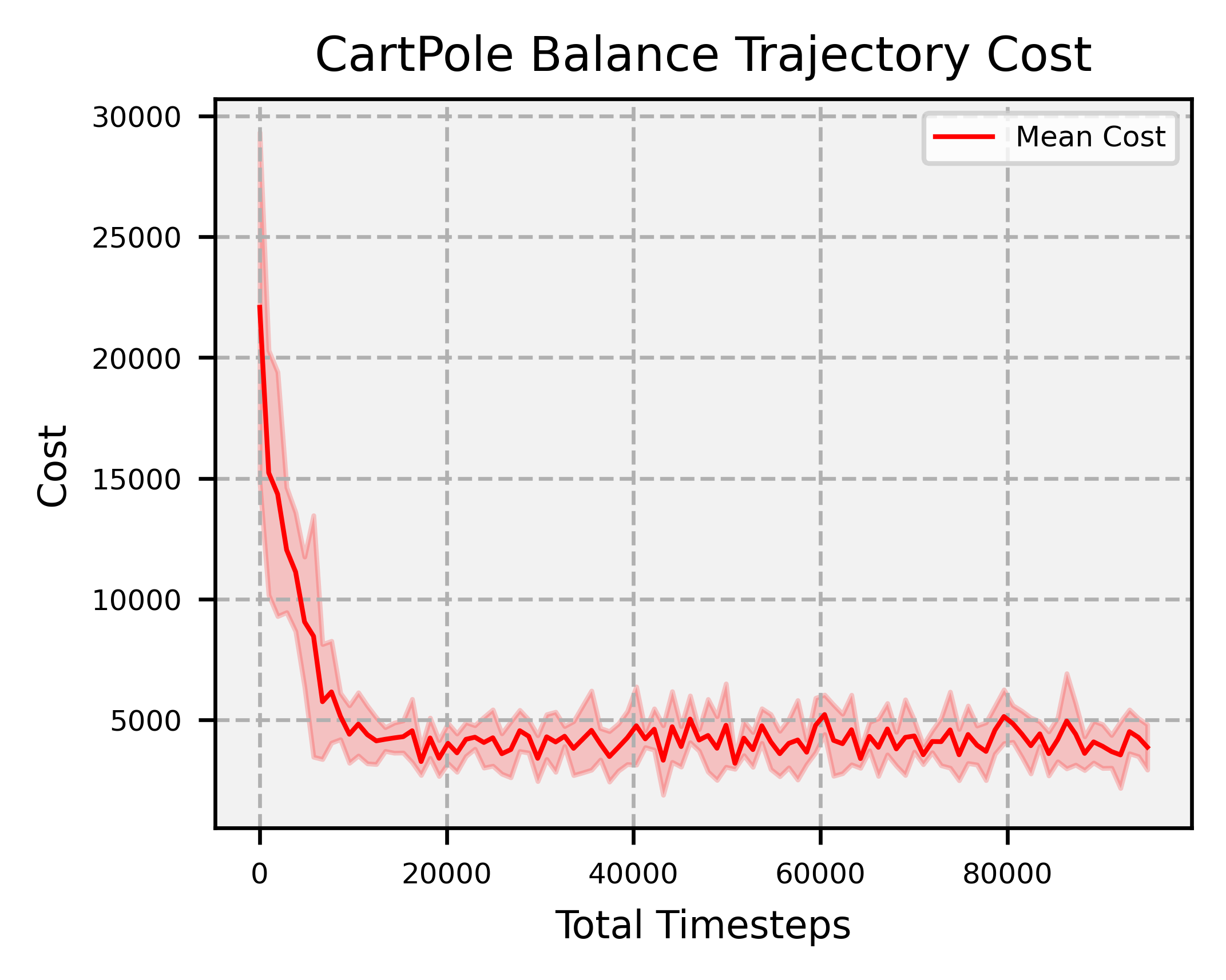
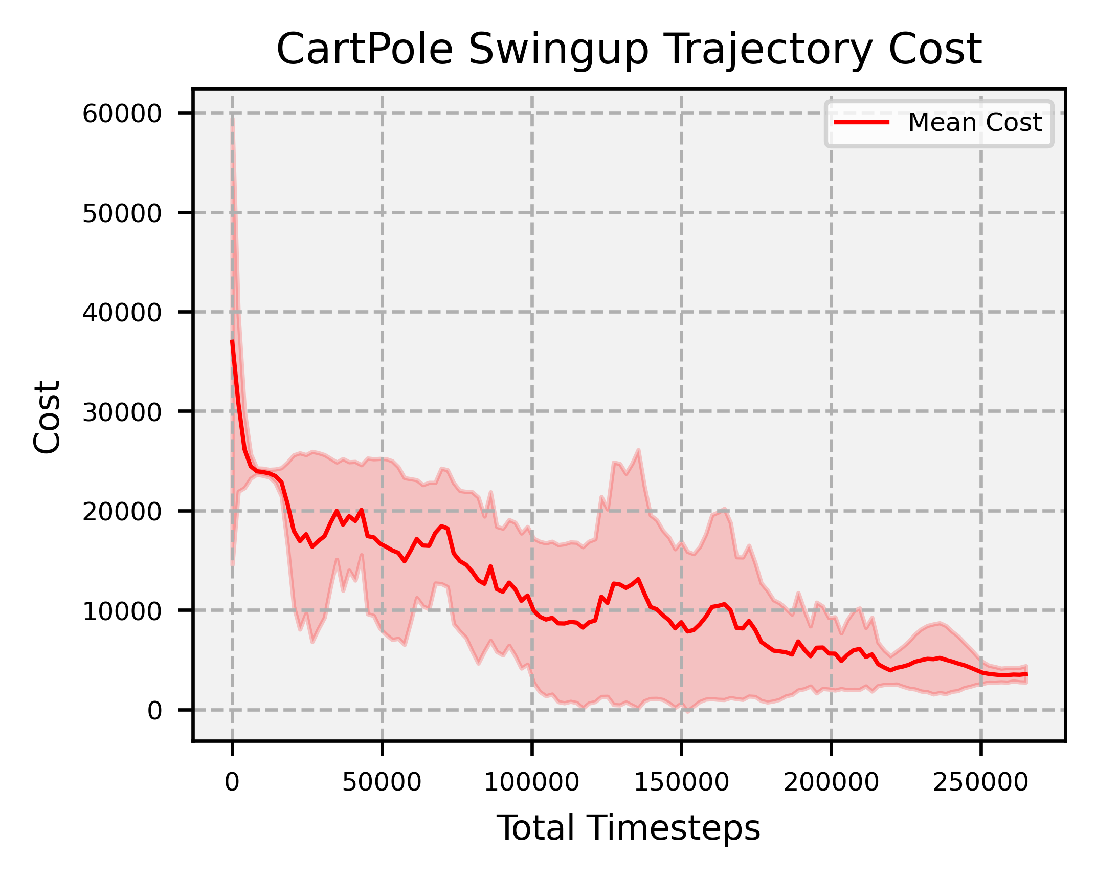
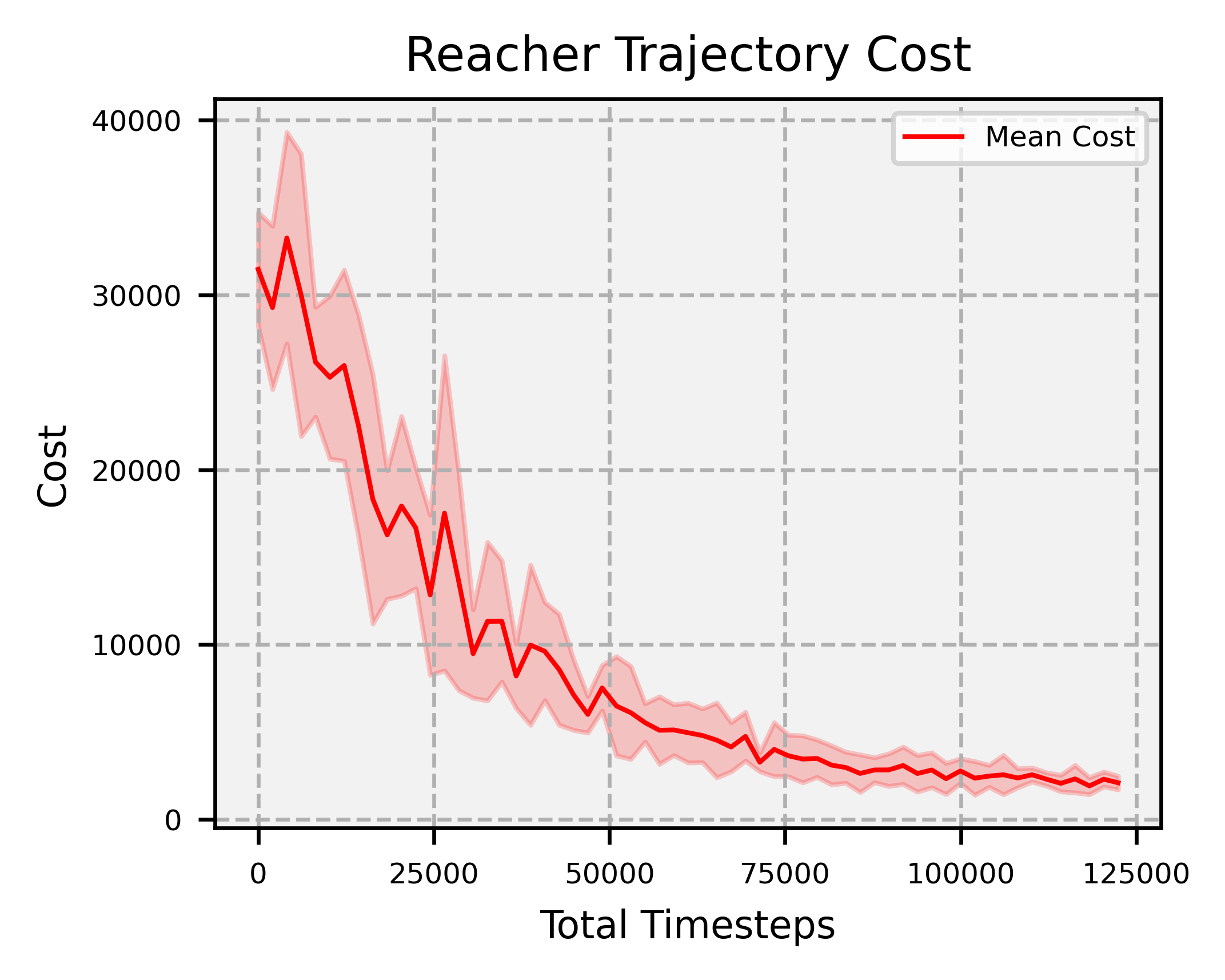
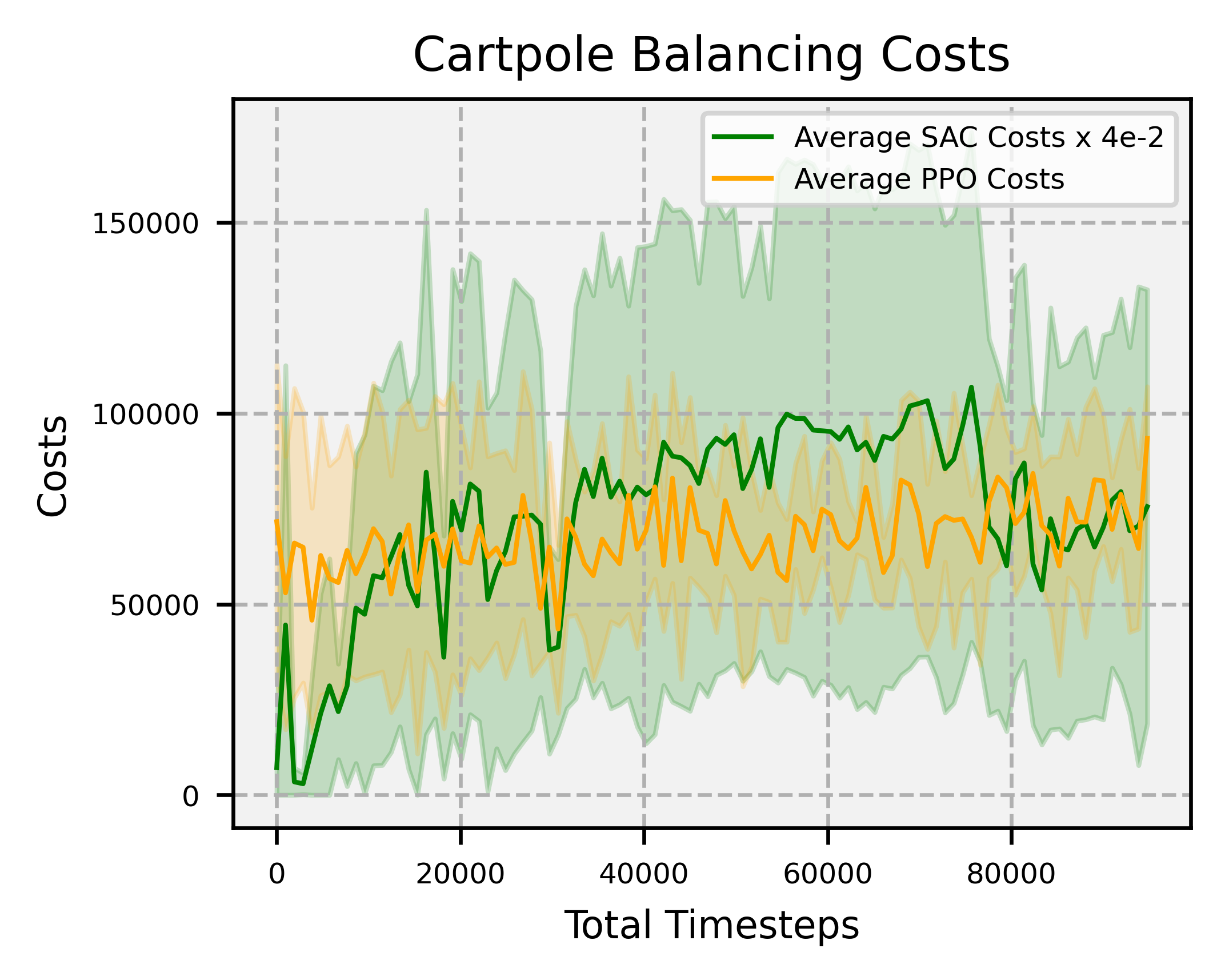
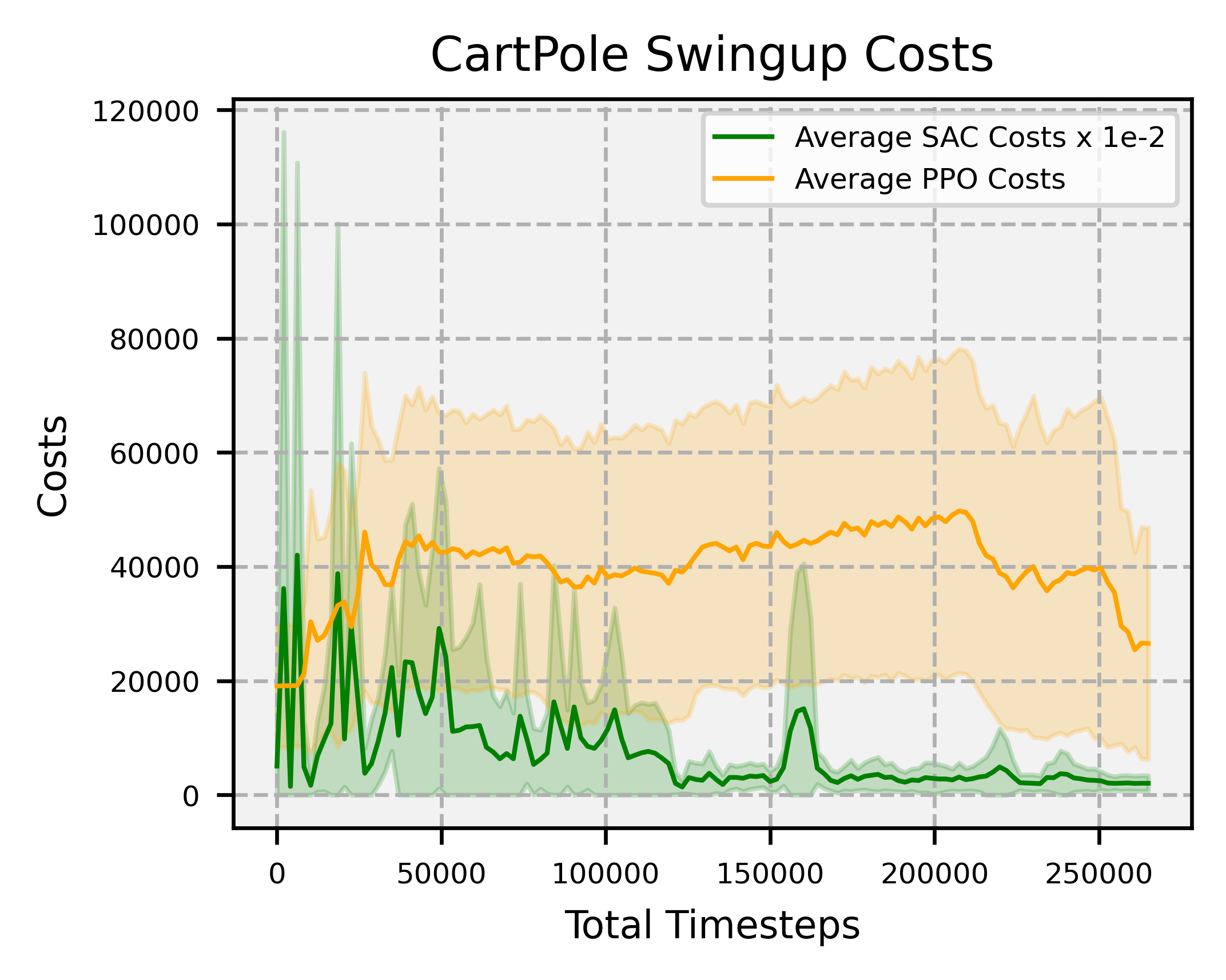
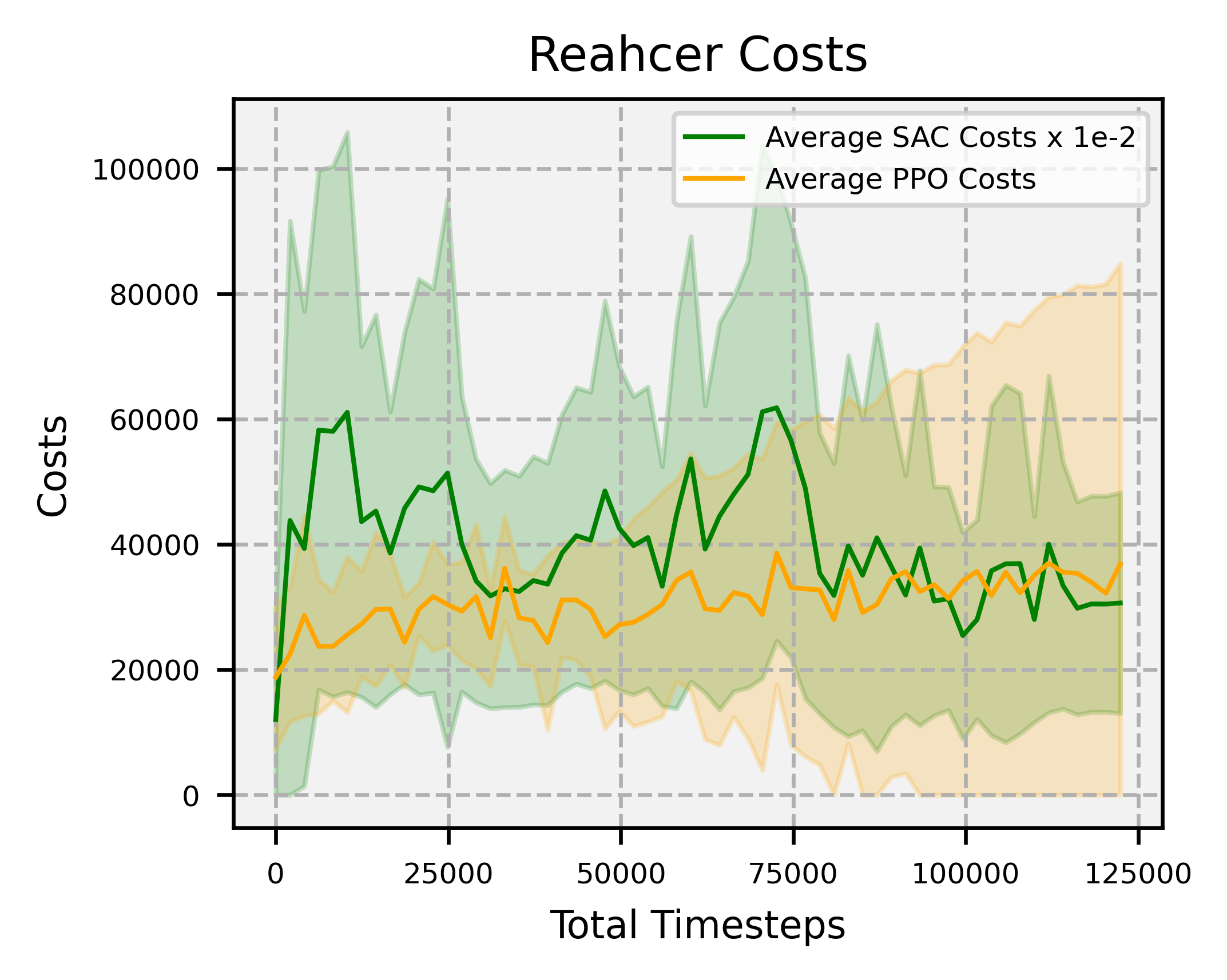
Overview: significantly faster convergence and lower variance across random seeds, outperforming SAC and PPO by factors of at least 74 and 2, respectively.